Web Neural Network Models (WebNNM)

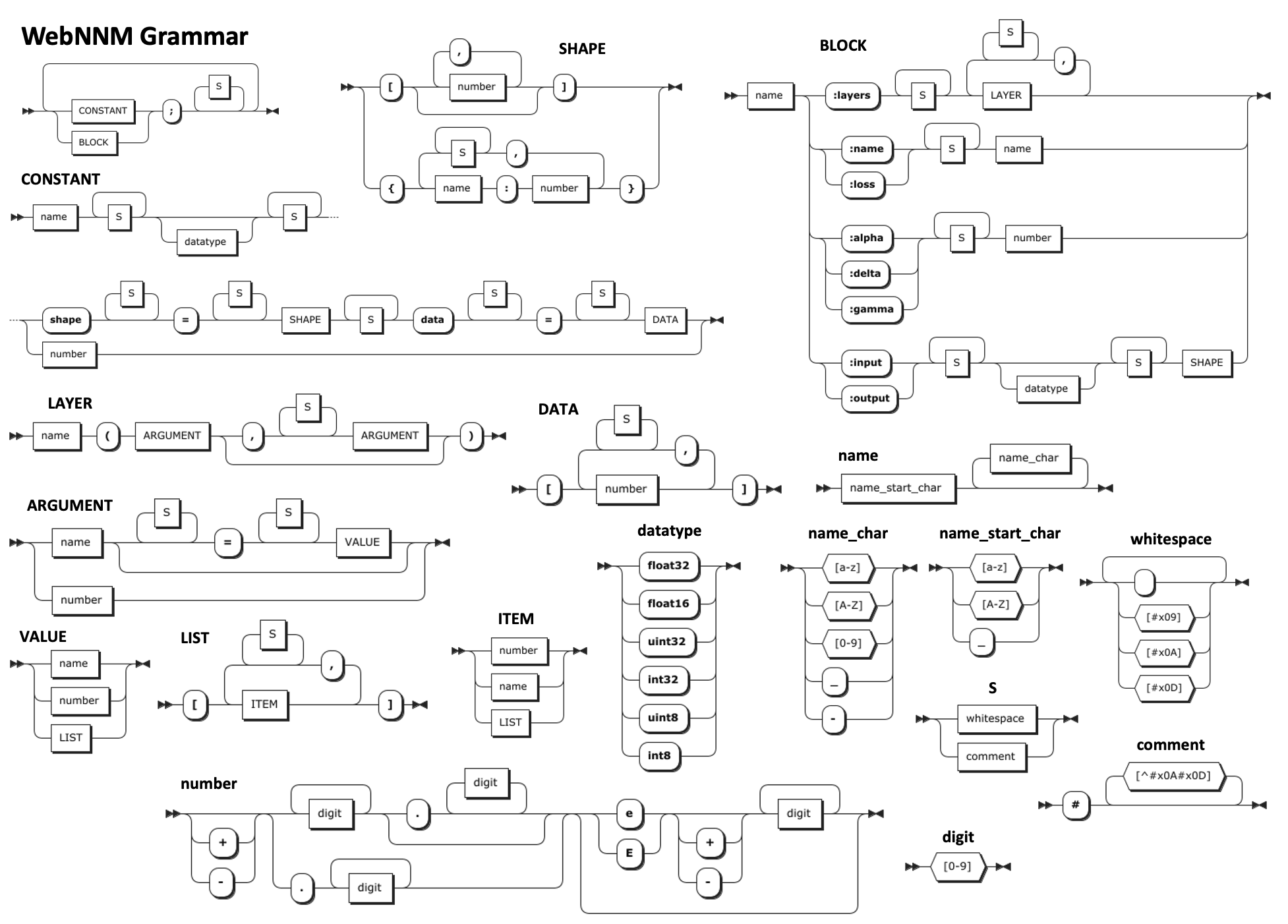
Existing neural network frameworks are huge and hard to use. WebNNM is a lightweight easy to understand high-level framework with an embedded expert system that simplifies working with neural networks for newcomers whilst offering experts fine grained control. This specification defines a high-level format for neural network models, and the API exposed by the associated JavaScript library. For an introduction and links to web-based demos, see [[WEBNNM-INTRO]].

This document reflects implementation experience, but is still subject to change. Feedback is welcome through GitHub issues or on the public-cogai@w3.org mailing-list (with public archives).

The grammatical rules in this document are to be interpreted as described in [[[RFC5234]]] [[RFC5234]].

Conformance classes

Conformance to this specification is defined for five conformance classes:

WebNNM model: A serialization of a [=neural network model=] as a file. A [=WebNNM document=] is conformant to this specification if it follows the grammar described in .
WebNNM snapshot: A serialization of a model and its parameters as a binary file. A [=WebNNM snapshot=] is conformant to this specification if it follows the format described in .
WebNNM authoring tool: An application that writes a [=WebNNM document=]. An [=authoring tool=] is conformant to this specification if it writes a conforming [=WebNNM document=].
WebNNM parser: A [=parser=] transforms a [=WebNNM document=] into another representation. A [=parser=] is conformant to this specification if it accepts any conforming [=WebNNM document=].
WebNNM Library: A software library that exposes the [=WebNNM API=] conforming to this specification.

Blocks and Layers

WebNNM seeks to make life easier for novices whilst providing experts with the control they seek. To realise this ambition, models are expressed in a high-level notation that uses meaningfully named tensor dimensions and omits batch size and sequence lengths, which are applied when compiling models into executable WebNN graphs or on export to MLIR. This allows tensors to be adapted to match the layouts provided by the datasets. The models only need to deal with feature layout, e.g. [channels, height, width] for images. Using meaningfully names makes layers easier to understand than the integer indices expected by WebNN.

WebNNM models are defined as a set of blocks, where each block has a set of properties, including a sequence of layers.

Here is an example with a model block that declares an input and an output, along with a sequence of dense layers. These are in turn defined by the dense block as a sequence of layers that multiply the input by a matrix, add a bias and apply an activation.

mode:name basic-model;
model:input shape=[784];
model:output shape=[10];
model:layers 
    dense(shapes=[[128],[80],[40]], activation=relu),
    dense(shape=[10], activation=softmax);
dense:layers
    matmul(w),
    add(b),
    activation();

Each layer has an operator, e.g. matmul, and zero or more operands followed by zero or more options. In this example, shapes, shape and activation are options. The shapes option signifies that a layer is to be repeated using the corresponding tensors shapes. In this case, a dense layer with output shape [128], a second with shape [80] and a third with shape [40]. WebNNM uses macros to bind options and their values. This is used to bind the activation to "relu" or "softmax". w and b are operands used to name model parameters. Note that the tensor shapes are declared excluding the dimensions for the batch size or sequence length, which are bound later. You are free to declare the data types if needed. The default data type is float32, subject to type inference. WebNNM applies tensor data type and shape inference, removing the need to explicitly specify the shape for every layer.

The permitted datatypes are taken from [[WebNN]]: float32, float16, int32, uint32, int8, uint8, int4, and uint4 (in order of decreasing precision). Note that [[WebNN]] places further restrictions on which data types can be used for certain operators. In addition, [[WebNN]] uses int32 for the size of each dimension, limiting it a maximum of 2147483648.

WebNNM applies inference from the inputs and outputs. Automatic data type casts are applied when needed from a lower to a higher precision, e.g. float16 to float32, but not from a higher to a lower precision. Note that type casting is applied lazily from the inputs to the outputs, i.e. preserving the lower precision until a cast to a higher precision is required. If you need greater control, you can provide explicit data types on the layers of interest.

Block input and output properties are expressed as the block name, followed by a colon then "input" or "output" respectively. This is followed by an optional data type and then a required shape, e.g. model:input float16 shape=[784]. Block properties are terminated with a semicolon. Layers are comma separated. The block name property is used when saving a snapshot. Blocks should name the dimensions when an input or output has more than one dimension, e.g. model:input float32 shape={channels:3, height:28, width:28};. The default dimension name is features for inputs and labels for outputs. The dimension names must be unique, and avoid reserved names: batch, and sequence. The choice of curly braces for shapes with named dimensions is deliberate, and resembles the distinction between JavaScript objects and arrays. Use square brackets for shapes without dimension names.

Named constants can be declared and referred to from layers. Here is an example of declaring constants named "pi", "foo" and "bar":

    pi float32 3.1415926;
    foo int32 shape=[4] data=[1, 1, 0, 0];
    bar shape={a:2, b:3} data=[0, 1, 2, 3, 4, 5];

where pi is defined as a scalar and bar as a rank 2 tensor with layout [a, b]. You have the choice of using curly braces with named dimensions or square brackets for just the dimension sizes.

I want to use icons to clearly distinguish trainable from non-trainable parameters, e.g. 🎓 and 🔒, but do I need the latter? The names given for trainable parameters are checked to see if they match layer names. If not the name is used as a prefix by gensym, e.g. "w" becomes "w1" or "w2" etc. Layer names are declared with the layer name option and gain suffices when a layer is cloned by instantiating a block and injecting its layers. Non-trainable parameters are inline literals or names for shared definitions. Model developers are encouraged to use naming conventions that clearly separate trainable parameter names from layer names.

Tensor Layout

WebNNM allows users to focus on the features and labels for their data, leaving the batch size and sequence length to be automatically applied when compiling to WebNN. The tensor layout defines how data is physically ordered in the computer's memory. Each tensor has a sequence of dimensions, e.g. [batch, features], or [batch, sequence, features] for sequenced data. The features themselves may be split across several dimensions, e.g. [batch, channels, height, width]. The tensor rank is the number of dimensions. The tensor size is the product of the dimension sizes. The tensor shape is the list of dimension sizes, e.g. [20, 3, 256, 256]. With a few exceptions, most layers preserve the layout. Here is a table showing variety of layouts and their applications:

Format	Structure	Primary Domain	Hardware Advantage
Batch-First	$B \times S\times F$	Transformers, General NLP	Intuitive for batch slicing and token-level operations.
Sequence-First	$S \times B \times F$	RNNs, LSTMs, Seq2Seq	Optimizes time-step looping memory access.
Channels-First	$B \times F \times S$	1D Convs, Audio, Time-Series	Fits legacy CuDNN convolution optimization.
Packed / Ragged	$TokenCount \times F$	LLM Serving, GNNs	Eliminates padding waste for variable lengths.

WebNNM automatically tracks the layout across the neural network, and applies any changes made by each layer. This is used to translate from dimension names for features to the integer indices in the full layout for the tensors operated on by WebNN.

Directed Acyclic Graphs

WebNNM parses to an object model for blocks and layers, and from there to a directed acyclic graph (DAG) with node types for inputs, outputs, parameters, literals and WebNN operations. Each node has an explicit data type and tensor shape. Nodes that are not on a path from an input node to an output node are culled, along with associated parameters and literals. Higher level operations are decomposed into WebNN operations as part of the process of building the DAG. Parameter nodes are annotated with attributes relating to how their tensors should be initialised based upon the activation function, for instance the Glorot or He algorithms, as well as good initial values for bias parameters.

The DAG is used to build executable WebNN graphs on demand for inference, testing and training. For testing, the dataset provides a sequence of batches of test data where the last batch may be smaller than the rest. The testing graph uses masking to ignore the missing data in the last batch. Training is similar. The training graph starts with a forward pass to compute the loss, then a backwards pass to compute the gradient of the loss with respect to each model parameter. This is followed by an optimizer that computes updates for the model parameters along with their momentum. A ping/pong approach is used to retain parameter values in the GPU or NPU's memory until training is complete. Further details are given in a later section. Note that DAG nodes omit the batch size and sequence length allowing the batch size, sequence lengths and full layout to be dynamically selected according to the needs of the dataset.

WebNNM Expert System

WebNNM aims to make things easy for newcomers whilst giving expert users the control they seek. An expert system auto-configures hyperparameters unless explicitly overriden, along with providing warnings about potential problems.

Comparison with other frameworks

WebNNM iterates through the DAG to build a profile of the network (e.g., looking for normalization layers, dropout, and counting parameter-heavy operations). The profile is mapped against the provided hyperparams to either auto-configure settings or emit warnings. Here is a comparison with other neural network frameworks:

Feature	WebNNM	Keras (TF/JAX)	PyTorch Lightning	TensorFlow.js
Philosophy	Expert-Guided: Proactively analyzes the DAG to fix common pitfalls.	User-Centric: Provides building blocks; leaves stability to the user.	Research Abstraction: Removes boilerplate but requires manual config.	Deployment First: Focuses on running models; training is secondary.
Regularization	Capacity-Aware: Auto-enables L2 if a high-capacity model lacks Dropout.	Manual / Granular: Must be added per-layer (kernel_regularizer).	Optimizer-Linked: Usually manual via weight_decay in the optimizer.	Manual: Required per-layer; no global "auto-regularize" logic.
Gradient Stability	Automatic (DAG-based): Detects depth/norms to enable AGC or Global Norm.	Manual: User must manually add clipping to the optimizer.	Configurable: User sets flags; framework doesn't "suggest" values.	Manual: Very low-level; no "auto" scaling/clipping.
Precision (float16)	Adaptive: Auto-scales based on model data types and DAG risk.	AMP: Efficient, but doesn't "warn" about specific layer risks.	AMP Toggle: Simple toggle; no topological analysis of risk.	Semi-Manual: Requires manual casts and precision management.
Multimodal Loss	Auto-Balanced: Avoids underflow by learning relative weights automatically.	Manual: User must provide a dictionary/list of weights.	Manual: Logic is typically buried in the training_step.	Manual: Verbose implementation for multi-output loss.

Breakdown of the Heuristics

Loss Functions: Recommends the loss function based upon the final activation layer, the training label's tensor shape and data type, and an examination of a sample batch of training data. Warns when the user's choice of loss function is inappropriate due to a mismatch between the loss function and the data it will receive.
Dynamic Gradient Scaling: In WebNN, leveraging $float16$ is one of the best ways to get speedups, but the gradients can easily fall below the minimum representable positive value of $float16$ ($\approx 5.96 \times 10^{-8}$). WebNNM examines the ratio of $float16$ vs $float32$ heavy layers. If the network is primarily running its dense operations in $float16$, it auto-enables dynamic gradient scaling to protect the narrow dynamic range. If the user selects $float16$ but turns scaling off, it's almost guaranteed to stall, hence the strong warning.
Gradient Clipping (AGC vs. Global Norm): Standard deep networks benefit from Global Norm clipping. However, if the DAG scan reveals a deep network (maxDepth > 15) but no normalization layers, it recommends/sets Adaptive Gradient Clipping (AGC). This is a nod to architectures like DeepMind's NFNets (Normalizer-Free Networks), where AGC is required to train without Batch Normalization.
Regularization: The system conducts a structural audit of the DAG to deploy an intelligent regularization strategy that balances Generalization (L2) with Sparsity (L1) based on the model’s "High Capacity" profile—a metric derived from depth, width, and the count of parameter-heavy operators. If a model lacks a sufficient "safety net" (a Dropout Density below 0.2), the system automatically enables L2 Regularization to prevent weight explosion and training data memorization. Furthermore, if the system detects a "Massive Input" (over 5,000 features), it injects L1 Regularization to act as a noise-gate, pruning irrelevant dimensions through feature selection. This dual-layered approach ensures that high-dimensional data and deep architectures remain stable and compressible, providing smart defaults for newcomers while supporting the control required by experts.
Targeting Vulnerable float16 Ops: It explicitly flags layers like softmax, log, exp, and normalizations (which calculate variance via sum-of-squares). The maximum value representable in $float16$ is 65504; operations like $e^x$ easily blow past this limit, resulting in NaNs propagating backward through your DAG. Grouping the warnings prevents console spam.
NPU Gentle Nudging: By counting how many heavy parameters (matmul, conv2d) are lingering in $float32$, WebNNM can issue a single aggregate recommendation to the user. This bridges the gap between experts (who might want $float32$ precision explicitly) and newcomers (who might not realize their battery is draining because they missed an optimization opportunity).
Uncertainty-Based Loss Weighting: Balances multimodal/multi-task outputs, treating each output's relative scale as a learnable weight ($s_i$) optimized directly within the WebNN graph. This approach is essential because mismatched loss magnitudes (e.g., MSE vs. Cross-Entropy) can cause dominant tasks to "drown out" others, especially in $float16$ environments where underflow is a constant risk. By automating this balance via homoscedastic uncertainty, the model dynamically stabilizes the gradient flow without time-consuming manual tuning. This remains highly efficient for consumer NPUs as it eliminates CPU-GPU synchronization and provides per-task numerical scaling, ensuring all tasks contribute effectively to training.

For consumer grade equipment, NPUs often support $float16$ but not $float32$. To speed training and prolong battery life, it is desirable to enable WebNN to use the NPU where practical through the use of $float16$ where this doesn't detract from training stability. WebNNM supports automatic casting and switches to $float16$ for critical operations. Note that WebNNM does not support $bfloat16$ although that may be added in future if and when it is added to WebNN.

WebNNM Application Programming Interface

This section describes the API for inference, testing and training, along with the API used for datasets.

Here is an example that declares a model and then tests it using a simple dataset.

import {NNModel} from "../webnnm.js"; // import WebNNM library
import * as Iris from "./datasets/iris-dataset.js"; // import an example dataset
    
window.addEventListener("load", async () => { 
    let dataset = await Iris.Dataset.create('./datasets/iris-dataset.csv');

    const source = `
        model:name test-model;
        model:loss categoricalCrossEntropy;
        model:input shape=[4];
        model:output shape=[3];
        model:layers 
            dense(shape=[3], activation=relu),
            dense(shape=[3], activation=softmax);
        dense:layers
            matmul(w),
            add(b),
            activation();
	`;

    const config = {
        source: source,  // or set url property to load from server
        dataset: dataset,
    };

    const model = await NNModel.create(config);
    
    await model.test(); // evaluate using dataset cited in config
});

The example starts with importing the WebNNM module and a dataset module. The application logic is called when the web page has finished loading. Note that the load event handler is marked as async, which is essential for subsequent use of await within the handler. The handler creates an instance of the dataset and declares the WebNNM model. These are passed to the NNModel.create() to create an instance of the model and bind it to the dataset. Finally, the application calls model.test() to apply the test subset of data provided by the dataset. Note that the WebNNM library calls the log function to log messages. This function defaults to console.log, but can be overridden by the application to log messages to the web page.

Inference

This section describes the API for inference.

Here is an example that declares a model and and runs it.

import {NNModel} from "../webnnm.js";

window.addEventListener("load", async () => { 

    const source = `
        model:name test-model;
        model:input int32 shape=[5];
        model:output float32 shape=[5];
        model:layers
            add(1, dataType=float16), 
            pow(2);
	`;

    const config = {
        source: source,  // or set url property to load from server
    };

    const model = await NNModel.create(config);

    // get a fresh inference context with default batch size of 1
    const context = await model.createContext();
    
    // initialise model input to 1
    let input = await context.setData([1, 2, 3, 4, 5]);
    
    // run model with the inference context
    await model.run(context);
    
    const output = await context.output();
        
    log(``);
    log(`input = ${model.view(input)}`);
    log(`output = ${model.view(output)}`);
});

The example starts with int32 for the input tensor and progressively casts it to float16 and finally to float32 for the output tensor. Note the use of numeric literals for operands for the add and pow operations.

The application calls model.createContext() to create a context object for inference. This object is used to initialise the input tensor before calling model.run(context) to create and execute the inference graph. context.output() is then used to retrieve the output tensor. Note the use of model.view() as a convenience function for logging tensors.

Context object methods:

setBatchSize(batchSize): Set the inference batch size, default = 1.
async input(name): Get the named input, defaults to first input.
async output(name): Get the named output, defaults to first output.
async randomize(blockName, lower, upper): Initialise input with named block to random numbers between lower and upper. If the block name is missing, it will initialise the first input. Default is -1 for lower and +1 for upper.
setData(blockName, data): Set input for named block from an array of numbers. If the block name is missing, it will initialise the first input. The data must be an array of numbers with the number items equal to the tensor size.

Testing

This section describes the API for testing.

Here is an example that declares a model and and run the test data on it.

import {NNModel} from "../webnnm.js"; // import WebNNM library
import * as Iris from "./datasets/iris-dataset.js"; // import an example dataset
    
window.addEventListener("load", async () => { 
    let dataset = await Iris.Dataset.create('./datasets/iris-dataset.csv');

    const source = `
        model:name test-model;
        model:loss categoricalCrossEntropy;
        model:input shape=[4];
        model:output shape=[3];
        model:layers 
            dense(shape=[3], activation=relu),
            dense(shape=[3], activation=softmax);
        dense:layers
            matmul(w),
            add(b),
            activation();
	`;

    const config = {
        source: source,  // or set url property to load from server
        dataset: dataset,
    };

    const model = await NNModel.create(config);
    
    await model.test(); // evaluate using dataset cited in config
});

model.test(): runs the testing graph on the testing subset of the dataset.

Training

This section describes the API for training.

Here is an example that declares a model and and trains it on the training data.

import {NNModel} from "../webnnm.js"; // import WebNNM library
import * as Iris from "./datasets/iris-dataset.js"; // import an example dataset
    
window.addEventListener("load", async () => { 
    let dataset = await Iris.Dataset.create('./datasets/iris-dataset.csv', {});

    const source = `
        model:name test-model;
        model:loss categoricalCrossEntropy;
        model:input shape=[4];
        model:output shape=[3];
        model:layers 
            dense(shape=[3], activation=relu),
            dense(shape=[3], activation=softmax);
        dense:layers
            matmul(w),
            add(b),
            activation();
	`;

    const config = {
        source: source,  // or set url property to load from server
        dataset: dataset,
    };

    const model = await NNModel.create(config);
    
    // training using training subset of data
    await model.train({
        epochs: 5000,
        optimizer: 'rlion',
        seeds: 50,
    });
    
    await model.test(); // independent assessment using testing subset of data
});

Training Hyperparameters

Training is similar to testing, but involves a set of training hyperparameters, so called to avoid confusion with the model's trainable parameters:

model.train(hyperparameters): runs the training graph on the training subset of the dataset.

hyperparameters is an object with the following optional properties:

epochs: the maximum number of epochs to train, default = 20
lr: the maximum learning rate, where the default depends on the choice of optimizer
warmupEpochs: for cosine annealing, use 0 to auto-calculate based on total epochs, default: 0
seeds: the number of seeds to scout to evaluate potential starting points for training, default: 100
patience: the maximum number of epochs to continue after minium loss, default: 500
lossWeights: to weight outputs when computing the epoch loss, default is 'auto' for automatic weighting
optimizer: name of the learning rate optimizer: 'lion', 'rlion', 'nesterov', or 'sgdm', default: 'rlion'
weightDecay: an attribute for learning optimizers, default depends on optimizer
momentumFactor: an attribute for the sgdm optimizer, default depends on optimizer
beta1: an attribute for the lion and rlion optimizers, default depends on optimizer
beta2: an attribute for the rlion optimizer, default depends on optimizer
freeze: what proportion of the layers to freeze for transfer learning (0.0 to 1.0) default: 0.0
regularization: 'auto', L1', 'L2', ''L1+L2' or 'off', default: 'auto'
lambda1: weight for L1 regularization, default: zero
lambda2: weight for L2 regularization, default: zero
optimizeFor: 'size' or 'edge', default: 'size'
gradientScaling: 'auto', 'on' or 'off', default: 'auto'
gradientClipping: 'auto', 'global', 'agc' or 'off', default: 'auto'
scale: initial gradient scaling factor, default = 1000
growthInterval: number of batches before increasing scale factor, default: 1000

Validation, testing and learning rate optimizers

The model parameters are validated after each epoch if the dataset provides a validation subset. On detecting a minima in the loss, the model weights are saved, and training continues for a given number of epochs. The training loss is reported every 50 epochs. Applications should always test the model when training completes. Testing the model on independent data after training is essential to verify that the network has truly learned generalizable patterns rather than simply memorizing the training data.

WebNNM supports a choice of learning rate optimizer. The choices all involve tracking the gradient and its momentum for each of the model parameters:

EvoLved Sign Momentum (lion): A memory-efficient stochastic gradient descent method discovered by Google. Unlike Adam, which tracks both first and second-order moments, Lion only tracks momentum. It uses the sign operator on the momentum to determine the update direction, allowing for a smaller memory footprint and often better performance at large batch sizes.
Refined Lion (rlion): Improves upon the original Lion optimizer by replacing the discrete sign function with a continuous, non-linear bounded function, yielding more stable updates. WebNNM uses softsign in place of arctan, which isn't supported by WebNN.
Nesterov Accelerated Gradient (nesterov): An advanced momentum-based optimizer that improves upon standard gradient descent by incorporating a "look-ahead" mechanism. Instead of calculating the gradient at the current parameter position, it computes the gradient at the position where the parameters will be after applying the current momentum velocity. This anticipation allows the algorithm to correct its course more effectively, leading to faster convergence and reduced oscillations.
Stochastic Gradient Descent with Momentum (sgdm): A popular optimization algorithm that enhances standard Stochastic Gradient Descent (SGD) by adding a momentum term. This term accumulates an exponential moving average of past gradients to accelerate convergence, help navigate narrow valleys, and avoid getting stuck in shallow local minima.

Scouting for good starting points

Training can be rather time consuming, so it makes sense to avoid waisting time when the initial choice of model parameter values doesn't train well. WebNNM creates a scouting graph to evaluate a set of randomly chosen potential starting points using a few heuristics. The metrics include: Loss, Gradient Ratio, and Dead Ratio. The gradient ratio detects vanishing or exploding gradients, whilst the dead ratio detects dead neurons or overconfident layers.

Cosine Annealing

WebNNM manages training in terms of a warm up phase in which the learning rate is gradually increased to the maximum learning rate. After that the learning rate is gradually reduced using cosine annealing to a very low value when reaching the maximum number of epochs. The default value for warmupEpochs is 5% of the maximum number of epochs, or 1, whichever is larger.

Multimodal/Multi-task Models

Multimodal models combine different modalities, e.g. video and audio. Multimodal models provide superior accuracy and robustness by leveraging redundant information and cross-sensory context to resolve ambiguities that a single data source cannot. Multi-task models are trained on multiple objectives from a shared representation. WebNNM allows you to specify the relative weights of each modality (or task) to avoid one modality drowning out the learning signals for another, especially in $float16$ environments where underflow is a constant risk. WebNNM addresses this challenge using Uncertainty-Based Weighting. Each task $i$ is assigned a learnable log-variance $s_i$. The total loss $L$ is computed as:$$L = \sum_i \left( \frac{1}{2e^{s_i}} L_i + \frac{1}{2}s_i \right)$$ This allows the optimizer to dynamically attenuate noisy tasks. To ensure stability in $float16$, $s_i$ is initialized at $0.0$ and a gradient scale $S \ge 128$ is recommended.

Transfer Learning

WebNNM supports transfer learning by allowing you to freeze parameter updates for the early layers of the network. This is based upon annotating each node in the DAG with the maximum number of nodes to reach an input node, and likewise to reach an output node. The freeze hyperparameter is a number in the range 0 to 1, defaulting to 0. It describes the proportion of layers to freeze, starting from the inputs. Parameters associated with nodes closer to the outputs are updated with a fraction that goes from 0 to 1 in a sinusoidal pattern (in range 0 to $\pi/2$). This range is discretised into 5 buckets to enable kernel optimization.

Training Stability

Training involves computing gradients that risk vanishing or exploding. For models with many layers it is good practice to introduce skip connections that bypass a few layers that would otherwise overly weaken the learning signals. It is common to use float32 whilst training to provide an adequate precision for gradients. However, the hardware accelerators in consumer grade equipment may not support float32, motivating the use of a lower precision, e.g. float16. This increases the risk of underflow and overflow during gradient calculations. Another consideration is that whilst GPUs can be used for hardware acceleration of neural networks, they consume considerably more electrical power than NPUs like Apple's ANE. To speed up training in the browser and reduce power consumption, it is desirable to find ways to increase training stability when using float16.

To address this challenge, WebNNM supports techniques to boost weak gradients, to scale down overly large gradients, and ignore updates that overflow the maximum number supported for a given precision. The scaling hyperparameter controls gradient scaling, whilst clipping controls clipping. If you set these to 'auto' (the default) the library examines the width and depth of the model along with the activation functions to assess whether to enable scaling and clipping. For explicit control set these hyperparameter to 'on' or 'off' as desired.

To prevent underflow during the backward pass, WebNNM multiplies the loss $L$ by a scale factor $S$ (where $S \gg 1$) before backpropagation begins. By the chain rule, this scales every subsequent gradient in the computational graph:$$\nabla_{\theta} (L \cdot S) = S \cdot \nabla_{\theta} L$$This ensures that the intermediate gradients $g$ that would have been $10^{-7}$ (and thus zeroed out in float16) are now $g \cdot S$, keeping them within the precision range. We cannot apply the scaled gradients directly to the model's parameters, as this would be equivalent to using a learning rate that is $S$ times too large. Before the optimizer updates the parameter $\theta$, the gradients need to be unscaled back to their original magnitude:$$\theta_{t+1} = \theta_t - \eta \cdot \frac{\sum \nabla_{\theta} (L \cdot S)}{S}$$

Use the scale hyperparameter to set the initial gradient scaling factor. The scale is doubled until overflow is detected at which point it is halved. To prevent instability, the growthInterval hyperparameter sets the number of batches without overflow to wait before boosting the scale factor. The forward and backward passes may use float16 for speed, but it is better to keep the model parameters in float32, and likewise to cast from float16 to float32 for operations like softmax and batchnorm. WebNNM will do this for you unless you explicitly set the data types in the model.

Clipping is based upon the scaled global (L2) norm $||\mathbf{G}||_2$ which is defined as the square root of the sum of the squares of every individual scalar value across all gradient tensors $g_i$:$$||\mathbf{G}||_2 = \sqrt{\sum_{i=1}^{n} \sum_{x \in g_i} x^2}$$

The training graph computes the rolling mean for the scaled global norm and its absolute deviation, as a basis for dynamically setting the clipping threshold:

Update mean: $\mu_{t} = \alpha \mu_{t-1} + (1 - \alpha) G$, where G is the current scaled global norm, and $\mu_0$ is set to the initial scaled global norm
Update deviation: $\sigma_{t} = \alpha \sigma_{t-1} + (1 - \alpha) |G - \mu_t|$, where $\sigma_o$ is set to zero
Compute dynamic threshold: $Threshold = \mu_t + (k \cdot \sigma_t)$
If $G > Threshold$, scale the gradients by $\frac{Threshold}{G+\epsilon}$, where $\epsilon$ is a very small positive number used to prevent the possibility of dividing by zero

Note that $k$ is 4.0 for the first 15 batches and 2.0 after that.

Work is underway to support automated gradient clipping (AGC) and regularization on a layer by layer basis.

Datasets

This section describes the API for datasets.

Supported Operators

This section lists the WebNN operators supported by WebNNM along with additional operators, e.g. for skip connections and transformers, that are internally translated into WebNN operators. Each operator's signature has a sequence of comma separated arguments, which are either order-dependent operands or order-independent properties of the form name = value.

Positional arguments = Tensors (The active data/operands flowing through the graph, whether they are constants, trained weights or previous layer outputs).
Named keyword properties = Structural Settings (The configurations that shape the network layout, like axis dimensions, strides, or hardcoded scaling limits).

The layer's input is implicitly the first operand. softmax(), thus has one operand, corresponding to the layer's input, whilst add(b) has two operands: the first is the layer's input and the second is the trainable parameter "b" which is given a unique numeric suffix when instantiated into the model's DAG. Names for constants and layers take precedence over parameters, e.g. if "pi" has been defined as a constant then mul(pi) will multiply the layer's input by the constant pi. Whilst operands are position dependent, options are position independent and can be given in any order. Options are non-trainable.

WebNNM seeks to make life easier for novices whilst providing experts with the control they seek. To realise this ambition, models are expressed in a high-level notation that uses meaningfully named tensor dimensions and omits batch size and sequence lengths, which are applied when compiling models into executable WebNN graphs or on export to MLIR. This allows tensors to be adapted to match the layouts provided by the datasets. The models will often only need to deal with feature layout, e.g. [channels, height, width] for images. Using meaningfully names makes layers easier to understand than the integer indices expected by WebNN.

WebNNM Operators

Operators inherited from WebNN:

Category	WebNN Operators
Tensor Creation	input, constant
Tensor Manipulation	concat, expand, gather, gatherElements, scatterElements, gatherND, scatterND, where, pad, reshape, slice, split, transpose, resample2d, reverse, tile, triangular
Tensor Quantization	quantizeLinear, dequantizeLinear
Tensor Casting	cast
Mathematics	add, sub, mul, div, max, min, clamp, pow, abs, ceil, cos, erf, exp, floor, identity, log, neg, reciprocal, sin, sqrt, tan, tanh, sign, clamp
Logical	equal, notEqual, greater, greaterOrEqual, lesser, lesserOrEqual, logicalNot, logicalAnd, logicalOr, logicalXor
Matrix Manipulation	matmul, gemm
Convolution	conv2d, convTranspose2d
Pooling	averagePool2d, l2Pool2d, maxPool2d
Activation	clamp, elu, gelu, hardSigmoid, hardSwish, leakyRelu, linear, prelu, relu, sigmoid, softmax, softplus, softsign, tanh
Normalization	batchNormalization, instanceNormalization, layerNormalization
Reduction	argMin, argMax, reduceL1, reduceL2, reduceLogSum, reduceLogSumExp, reduceMax, reduceMean, reduceMin, reduceProduct, reduceSum, reduceSumSquare, cumulativeSum
Recurrent Neural Networks	gruCell, gru, lstmCell, lstm

Note that you can write batchNorm in place of batchNormalization, and likewise instanceNorm and layerNorm.

Tensor Creation

The high-level model syntax caters for model inputs and outputs. Numeric literals can be used in place, or named and used elsewhere. Parameters are expressed as named operands for layers. Here are some examples:

model:input float16 shape={channels:3, height:256, width:256} An input for the model block with float16 for the datatype, and a shape for an image with named dimensions.
model:output float32 shape=[32] An output for the model block with float32 for the datatype and a shape with size 32, e.g. as a probability distribution across labelled classes.
matmul(w) A matmul layer with "w" as the trainable weight parameter. This will be given a unique suffix, e.g. "w1", when instantiated into the model's DAG to differentiate it from other instances. The data type and shape are determined automatically.
add(1.5) An add layer that adds the number 1.5 to the layer's input, using broadcasting to match the input tensor's shape.
pi float32 3.1415926 Declares "pi" as a named float32 scalar constant.
foo int32 shape=[4] data=[1, 1, 0, 0] Declares "bar" as the name of a constant int32 tensor with shape [4], and fill it with the listed values.
bar shape={a:2, b:3} data=[0, 1, 2, 3, 4, 5] Declares "foo" as the name of constant tensor with shape [2, 3] and layout [a, b]. The tensor is filled from the one dimensional buffer, which must have a length equal to the tensor's size, i.e. the product of the size of the tensor's dimensions, in this example, $size = 2 \times 3 = 6$

Tensor Manipulation

concat(tensor, tensor, ..., axis=name)

concat([tensor, tensor, ...], axis=name)

Concatenates the input tensors along a named axis. The operands is a variable list of tensors, which will be concatenated starting with the input from the previous layer. If you want to concatenate a list of tensors excluding the input from the previous layer, you must enclose the list in square brackets.

expand(newShape={...})

Expands any dimension of size 1 in the feature dimensions of the tensor from the previous layer to a larger size according to a target shape. The target shape is declared using curly braces. Inside the braces, dimensions targeted for expansion are specified with their name and a positive integer target size (e.g., channels:4). Dimensions that should be left unchanged are specified by their name alone (e.g., height), signaling to the compiler to inherit their size directly from the input tensor. Global dimensions like batch size and sequence length are omitted from this property and are automatically preserved by the backend. If the feature dimensions inside the braces are listed in a different order from the tensor passed from the previous layer, a transpose operation will be automatically inserted to permute the dimensions to match the exact layout order given in the layer.

gather(indices=tensor, axis=name)

This generates the output tensor by gathering all data for given positions along the named axis. The positions are relative to the start of the axis for positive indices, and relative to the end of the axis for negative indices. As an example, given an image, you could extract all pixels at the same height in the image. For this axis=height and indices is a single-valued array with the desired height index. You would generalise indices to a multi-valued array to pick pixels at selected heights. Gather copies the input dimensions before the target axis, then all of dimensions in the indices tensor, and finally the input dimensions after the target axis.

indices is a non-trainable n-dimensional tensor whose values are signed or unsigned integers. If $N$ is the size of the input dimension named by axis, then values must be in the range $-N$ (inclusive) to $N$ exclusive. The output tensor will have rank equal to the rank of the layer's input tensor plus the rank of indices minus 1. Models either declare the indices tensor as a named constant or generate it as the output of a named layer.

Some use cases involve gathering along the batch or sequence dimensions that are missing in the high-level model syntax, and dealt with when compiling to WebNN. Here is an example showing the run-time tensor shapes and layouts:

Input Shape: { batch: 32, sequence: 128, embedding: 768 }
Indices shape: { beam: 4, candidates: 2 }
Axis name: sequence
Output shape: { batch: 32, beam: 4, candidates: 2, embedding: 768 }
where the dimension named by axis has been replaced by the given shape.

Is it worth allowing indices to be defined in place in the layer? One way to do that would be to use shape and data properties as an alternative to indices, using the same syntax and meaning as for constant tensors. If adopted, this would also apply to gatherElements, scatterElements, gatherND and scatterND.

gatherElements(indices=name)

This operator acts like a target index map. It pairs each individual index with its exact coordinate location to pluck single, specific values from along the targeted axis. The indices tensor is subject to several constraints: a) it must have the same rank as the input tensor, b) every named dimension in the shape must match a dimension in the input, and c) for every dimension ‭‬that is not the target axis, the size in indices must be less than or equal to the size in input (usually they are identical). The layer's output shape and layout are the same as specified by the shape argument. Here is an example:

Input Shape: { batch: 32, sequence: 128, vocabulary: 50000 }
Indices shape: { vocabulary: 5 }
axis=vocabulary, e.g. getting top-5 beams
Output Shape: { batch: 32, sequence: 128, vocabulary: 5 }

Note that the batch and sequence dimensions are implicitly copied over from the input.

scatterElements(updates, indices=name, axis=name)

If gatherElements is about extracting data along an axis based on a map of indices, scatterElements (often used for things like sparse updates, scatter-add in graph neural networks, or applying target masks) is the exact inverse. It writes data from the updates tensor into a copy of the input tensor at the positions specified by the non-trainable indices tensor. The updates operand is either a trainable parameter, or the name for the output of another layer.

gatherND(indices=name)

The non-trainable indices array contains entire coordinates into the input tensor, with the rightmost dimension holding the number of dimensions per coordinate. So an indices tensor of shape [10,1] holds 10 single-axis coordinates, and a shape of [4,3] holds 4 indices of 3D coordinates. The values are integers in the range $-N$ (inclusive) to $N$ (exclusive), where $N$ is the is the size of the corresponding input dimension, and a negative index means indexing from the end of the corresponding dimension.

scatterND(updates, indices=name, axis=name)

Scatter slices of values from the updates tensor atop a copy of the input tensor according to the non-trainable coordinates. This operator is similar to gatherND with the addition of the updates operand which is either a trainable parameter, or the name for the output of another layer.

where(trueValue, falseValue, condition=tensor)

Selects the values from the trainable trueValue or falseValue tensors depending on the corresponding values of the non-trainable condition tensor, where non-zero is treated as true and zero as false.

pad(beginningPadding=list, endPadding=list, mode=string, value=integer)

Inflate the tensor with constant or mirrored values on the edges. beginningPadding is an array of length equal to the rank if the layer's input. Each value corresponds to the number of padding values to add before the content in that dimension. endPadding is similar, but applies to values added after the content in each dimension. The mode option is constant, edge or reflection. value is the padding value, with a default of 0. None of the pad layer arguments are trainable.

reshape(newShape={...})

Reshapes a tensor to a non-trainable new shape. The shape can be specified using curly braces to declare dimension names and sizes, or using square brackets for just the dimension sizes.

slice(starts=list, sizes=list, strides=list)

Produces a slice from the input tensor. starts lists the (zero based) starting index for each dimension. sizes correspondingly lists the number of elements to copy across from each dimension. The strides option lists the stride to step over each dimension in the input tensor. Stride must be zero or positive, and defaults to zero. None of the slice layer arguments are trainable.

split(splits=value, axis=name)

Splits the input tensor into a number of sub tensors along the given axis. splits is either a positive integer or a list thereof. In the former case, it must evenly divide the dimension size of the input tensor along the specified axis. If it is a list, each element specifies the size of the corresponding output tensor along the axis. The sum of sizes must equal to the dimension size of input along the axis. The axis option names the dimension along which to split, defaulting to the first feature dimension. None of the slice layer arguments are trainable.

transpose(permutation=[name, name, ...])

Permutes the dimensions of the layer's input tensor according to the given non-trainable permutation list, which lists all of the feature dimensions in the desired order. The compiler will automatically isolate and preserve global dimensions (like batch size and sequence length) in their original positions. For example, transposing a vision feature map from [height, width, channels] to [channels, height, width] automatically preserves the batch dimension at the front, achieving an NHWC to NCHW shift seamlessly.

For advanced use cases where a global dimension must be interleaved with feature dimensions—such as swapping the sequence and attention-head dimensions in a Transformer block ([batch, sequence, heads, depth] to [batch, heads, sequence, depth])—developers may explicitly include the names batch and sequence within the permutation list to override the compiler's automatic placement and gain full structural control of the runtime tensor. In this case the length of the permutation list must equal the full rank of the input tensor.

resample2D(newShape={...}, mode=modeName)

Resample the tensor values from the source to the destination dimensions according to the mode and scaling factors as determined by $scale = outputSize / inputSize$. The new shape associates the dimension names with the desired new size for that dimension. The mode name must be either nearest-neighbor or linear, defaulting to the former. The resample2D layer arguments are non-trainable.

Here is an example that resizes the image data to 64 by 64 pixels using bilinear interpolation:
resample2D(newShape={ height: 64, width: 64 }, mode=bilinear)

reverse(axes=[name, name, ...])

Reverses tensor data along non-trainable named axes.

Here is an example that flips the image left to right:
reverse(axes=[width])

tile(repetitions={...})

Repeat a tensor a given number of times along each non-trainable named dimension.

Here is an example that repeats the image twice vertically and three times horizontally:
tile(repetitions={ height: 2, width: 3 })

triangular(upper=boolean, diagonal=integer)

Given a 2-D tensor (matrix), return a 2-D tensor containing either the upper or lower triangular part of the input tensor. The upper property defaults to true and indicates whether to output the upper or the lower part of the input matrix. The diagonal property defaults to 0 and specifies an offset relative to the main diagonal of the matrix. A value of 0 means only elements bounded by the main diagonal itself are affected; a positive integer shifts the boundary up and to the right, while a negative integer shifts it down and to the left. Note that the operation applies to the last two feature dimensions. If these are not the final two dimensions in the run-time tensor layout, transpose operations will be automatically injected before and after the WebNN triangular operation. If the input tensor has greater than 2 dimensions it is treated as a batch of matrices and the result has the same shape. None of the triangular layer arguments are trainable.

Tensor Quantization

quantizeLinear(scale=name, zeroPoint=name): Quantizes a floating point tensor to an integer tensor using the scale and zero-point bias (e.g. output = clamp(roundEven(input / scale) + zeroPoint, 0, 255) for "uint8"). The scale and zeroPoint tensors can be smaller than the input tensor as they are blockwise broadcast. scale and zeroPoint name a layer, input or constant. The scale tensor values must be non-zero positive numbers. The zeroPoint tensor must have the same shape as the scale tensor. The layer's input data type must be float32 or float16. The data type of the scale tensor will (if needed) be casted to that of the layer's input. The data type for zeroPoint must be uint8, int8, uint32 or int32. The data type of the output is taken from the data type of zeroPoint.
dequantizeLinear(scale=name, zeroPoint=name): Dequantizes an integer tensor to floating point tensor using the scale and zero-point bias, where output = (input - zeroPoint) * scale. The scale and zeroPoint tensors can be smaller than the input tensor as they are blockwise broadcastable. scale and zeroPoint are defined in same way as for quantizeLinear except in respect to their data types. The layer's input data type must be uint8, int8, uint32 or int32. The same holds for zeroPoint. The data type of the scale tensor must be float32 or float16. The data type of the output is taken from the data type of scale.

Tensor Casting

cast(dataType=string): Cast each element in the input tensor to the target data type. dataType must be one of uint8, int8, uint32, int32, float16 or float32.
Some platforms may also support uint64 and int64.

Mathematics

The following are element-wise operations with two operands, where the first is the layer's input and the second trainable parameter is given as a layer argument (value).

add(value): The output is computed by adding the given value to the layer's input. value is a numeric literal or list thereof, or a name for a layer, input or constant. It will be broadcast as needed to match the layer's input.
sub(value): The output is computed by subtracting the given value from the layer's input. value is a numeric literal or list thereof, or a name for a layer, input or constant. It will be broadcast as needed to match the layer's input.
mul(value): The output is computed by multiplying the given value with the layer's input. value is a numeric literal or list thereof, or a name for a layer, input or constant. It will be broadcast as needed to match the layer's input.
div(value): The output is computed by dividing the layer's input by the given value. value is a numeric literal or list thereof, or a name for a layer, input or constant. It will be broadcast as needed to match the layer's input.
max(value): The output is computed by comparing the elements in the given value with those in the layer's input and taking the maximum. value is a numeric literal or list thereof, or a name for a layer, input or constant. It will be broadcast as needed to match the layer's input.
min(value): The output is computed by comparing the elements in the given value with those in the layer's input and taking the minimum. value is a numeric literal or list thereof, or a name for a layer, input or constant. It will be broadcast as needed to match the layer's input.
pow(value): The output is computed by raising the layer's input by power given by the value. value is a numeric literal or list thereof, or a name for a layer, input or constant. It will be broadcast as needed to match the layer's input.

Would it be worth allowing a list of operands in square brackets, where the layer's input is not an implicit member of the list? What are the use cases for adding more than two operands in this way?

The following are element-wise unary operations on the layer's input. The output has the same shape and data type as the input.

abs(): Computes the absolute value element-wise on the input tensor, stripping the negative sign from any numbers less than zero.
ceil(): Computes the ceiling element-wise on the input tensor, rounding each value upward to the nearest integer greater than or equal to the original value.
cos(): Computes the trigonometric cosine element-wise on the input tensor, expecting input values to be supplied in radians.
erf(): Computes the statistical Gauss error function element-wise on the layer's input tensor. It outputs a tensor of identical shape and data type, mapping all input values to a smooth curve bounded strictly between -1.0 and 1.0.
exp(): Computes the exponential function element-wise on the input tensor, raising Euler's number ($e$) to the power of each input value.
floor(): Computes the floor element-wise on the input tensor, rounding each value downward to the nearest integer less than or equal to the original value.
identity(): Returns a new tensor with the exact same shape and values as the input tensor, acting as a clean pass-through layer often used to force data routing or manage graph endpoints.
log(): Computes the natural logarithm (base-$e$) element-wise on the input tensor, strictly expecting positive input values.
neg(): Computes the numerical negation element-wise on the input tensor, effectively multiplying every element by -1 to flip its arithmetic sign.
reciprocal(): Computes the reciprocal element-wise on the input tensor, calculating $1 / x$ for every individual value.
roundEven(): Computes the round-to-nearest-even operation (also known as convergent or banker's rounding) element-wise on the input tensor. It rounds values to the nearest integer, but resolves halfway cases (e.g., 1.5 or 2.5) strictly to the nearest even integer to eliminate statistical accumulation bias.
sin(): Computes the trigonometric sine element-wise on the input tensor, expecting input values to be supplied in radians.
sign(): Extracts the sign element-wise on the input tensor, returning -1 for negative numbers, 0 for zero, and 1 for positive numbers.
sqrt(): Computes the square root element-wise on the input tensor, strictly expecting non-negative input values.
tan(): Computes the trigonometric tangent element-wise on the input tensor, expecting input values to be supplied in radians.

Finally, the clamp operator:

clamp(min=minValue, max=maxValue): Clamp the input tensor element-wise within a range specified by the minimum and maximum values. minValue and maxValue are optional numbers. If either are missing, the corresponding clamp is not performed. The output tensor of the same shape as input.

Logical

Logical operators generate a tensor with the data type uint8 with a non-zero value (usually 1) for true and zero for false. For operators with more than one operand, the operands are broadcast as needed. The shape of the output tensor is the same as the shape of the broadcasted input. The value argument is non-trainable.

equal(value): Compares two tensors element-wise and returns a boolean tensor of the same shape, where each position is 1 (true) if the corresponding elements are equal, and 0 (false) otherwise. Supports implicit broadcasting if the shapes differ.
notEqual(value): Compares two tensors element-wise and returns a boolean tensor of the same shape, where each position is 1 (true) if the corresponding elements are not equal, and 0 (false) otherwise. Supports implicit broadcasting if the shapes differ.
greater(value): Compares two tensors element-wise and returns a boolean tensor of the same shape, where each position is 1 (true) if the element in the primary tensor is strictly greater than the corresponding element in the other tensor, and 0 (false) otherwise. Supports implicit broadcasting if the shapes differ.
greaterOrEqual(value): Compares two tensors element-wise and returns a boolean tensor of the same shape, where each position is 1 (true) if the element in the primary tensor is greater than or equal to the corresponding element in the other tensor, and 0 (false) otherwise. Supports implicit broadcasting if the shapes differ.
lesser(value): Compares two tensors element-wise and returns a boolean tensor of the same shape, where each position is 1 (true) if the element in the primary tensor is strictly less than the corresponding element in the other tensor, and 0 (false) otherwise. Supports implicit broadcasting if the shapes differ.
lesserOrEqual(value): Compares two tensors element-wise and returns a boolean tensor of the same shape, where each position is 1 (true) if the element in the primary tensor is less than or equal to the corresponding element in the other tensor, and 0 (false) otherwise. Supports implicit broadcasting if the shapes differ.

The following operators expect their inputs to have the data type uint8:

logicalNot(): A unary operation that computes the logical inversion element-wise on an input boolean tensor, flipping all true values to 0 (false) and false values to 1.
logicalAnd(value): Computes the logical AND operation element-wise between two boolean tensors. Returns a boolean tensor where each position is 1 (true) only if the elements in both tensors are non-zero, and 0 (false) otherwise. Supports implicit broadcasting if the shapes differ.
logicalOr(value): Computes the logical OR operation element-wise between two boolean tensors. Returns a boolean tensor where each position is 1 (true) if at least one of the corresponding elements in either tensor is non-zero, and 0 (false) otherwise. Supports implicit broadcasting if the shapes differ.
logicalXOr(value): Computes the logical exclusive OR (XOR) operation element-wise between two boolean tensors. Returns a boolean tensor where each position is 1 (true) if the corresponding elements differ (one is non-zero and the other is zero), and 0 (false) if they are both zero or both non-zero. Supports implicit broadcasting if the shapes differ.

Matrix Manipulation

The matmul operator is used for fully connected dense layers in conjunction and the add operator: $y = W\cdot x + b$. In transformers, matmul is the core of the attention mechanism, computing the similarity of query and key matrices to produce attention scores. It also plays a frequent role in calculating gradients as part of machine learning.

matmul(value): Computes the matrix multiplication of the primary tensor (the layer's input) and the value tensor, as specified by the name of a trainable parameter, an input constant or another layer. The operation is applied strictly to the trailing two feature dimensions of both inputs (interpreting them as rows and columns of a matrix). If either tensor has a rank greater than 2, the leading dimensions (such as batch sizes or attention heads) are treated as batch dimensions and are automatically aligned and broadcasted by the compiler to match. The inner dimensions of the two matrices must match at run-time to satisfy standard linear algebra rules. If the targeted matrix dimensions are not at the trailing end of the resolved runtime layouts, the compiler will automatically inject transpose operations to ensure a safe WebNN compilation.
gemm(B, C, alpha=number, beta=number, aTranspose=boolean, bTranspose=boolean): Computes the General Matrix Multiplication (GEMM) expression $\alpha A B + \beta C$, combining a scaled matrix multiplication with a scaled bias tensor addition. The primary tensor (the layer's input) acts as matrix $A$, parameter B specifies matrix $B$, and an optional parameter C specifies the bias tensor $C$. The scalar multipliers alpha and beta both default to 1.0. The boolean flags aTranspose and bTranspose default to false; setting either to true instructs the WebNN backend to implicitly transpose the final two dimensions of the associated matrix ($A$ or $B$) prior to multiplication, which is highly optimized at the hardware level. Like matmul, this operation applies to the trailing two feature dimensions of the tensors, and any leading dimensions are automatically managed and broadcasted as batch matrices. Tensors B and C are trainable, alpha, beta and the transpose flags are not trainable.

Convolution

These operators are used in Convolutional Neural Networks (CNN) for learning, feature extraction and spatial manipulation. conv2d is used to extract local spatial features from input images. This includes edges, corners, textures, or higher-level patterns progressively through deeper layers. A small learnable kernel slides across the spatial dimensions of the input, computing weighted sums for each local region. This reduces spatial redundancy, emphasizing features useful for classification or recognition.

convTranspose2D performs learnable upsampling, expanding spatial dimensions of feature maps. It is the inverse of conv2d, spreading or broadcasting input activations across a larger area, and often used to reconstruct high-resolution outputs from compressed representations. It increases height and width while preserving learned features for generative tasks. It can introduce artifacts like checkerboarding if the stride and kernel configuration are not carefully chosen.

conv2d(filter, padding={height:number, width:number], strides={height:number, width:number}, dilations={height:number, width:number}, groups=integer, inputLayout=string, filterLayout=string): Computes a 2D spatial convolution by sliding a weight filter tensor across the input feature map to extract localized spatial features. The inputLayout string configures the expected ordering of the dimensions (nchw for channel-first or nhwc for channel-last), allowing the compiler to parse and map the global batch ($N$), channel ($C$), and spatial spatial ($H, W$) axes. Similarly, filterLayout specifies the structure of the weight tensor: iohw, hwoi or ohwi.

Optional tuning arrays include padding (explicit pixel boundaries added around the input, matching [top, bottom, left, right]), strides (the pixel stepping increment along the height and width, matching [height, width]), and dilations (the receptive field spacing between filter elements, matching [height, width]). The groups parameter partitions the input channels into independent calculation blocks for depthwise or grouped convolutions.
convTranspose2D(filter, padding={height:number, width:number], strides={height:number, width:number}, dilations={height:number, width:number}, outputPadding={height:number, width:number}, outputSizes={height:number, width:number}, groups=integer, inputLayout=string, filterLayout=string): Computes a 2D transposed convolution (sometimes referred to as a fractionally strided convolution or "deconvolution") to upsample spatial feature maps, a mechanic widely used in generative models and segmentation networks. The layout strings inputLayout and filterLayout map the dynamic runtime axes to WebNN exactly as they do in conv2d. The spatial upscaling scale is primarily determined by the strides array, which acts as a multiplier on the output canvas.

To resolve spatial ambiguity caused by integer division in stride math, developers can explicitly control the output canvas size using either outputPadding (extra pixels added to the bottom and right edges of the output tensor) or an explicit outputSizes layout block. The remaining parameters (padding, dilations, and groups) operate as the inverse of standard convolutional operations to govern weight spatial distribution.

Pooling

Pooling operations are used in Convolutional Neural Networks (CNN) to compress images while retaining the most important information. Pooling is applied after convolution layers for dimensionality reduction, translation invariance and feature selection. Progressively reducing the spatial dimensions, pooling layers enable the network to build a hierarchy of features. Lower layers capture fine details, while higher layers focus on more abstract and global features. The choice of pooling size, stride, and type needs to balance dimensionality reduction and feature preservation.

Each of the operators support the same options:

windowDimensions={height:number, width:number}: Specifies the dimensions of the sliding window. The default value for the window dimensions are the height and width dimensions of the input shape.
paddingBeginning={height:number, width:number}: Specifies the additional rows and columns added to the beginning of each spatial dimension of the convolution input. No padding is the default.
paddingEnding={height:number, width:number}: Specifies the additional rows and columns added to the ending of each spatial dimension of the convolution input. No padding is the default.
strides={height:number, width:number}: Specifies the additional rows and columns added to the beginning and ending of each spatial dimension of the convolution input. The default values are zero.
dilations={height:number, width:number}: Specifies the dilation factor for each spatial dimension applied on the convolution filter (kernel). The default value is one pixel.
layout=string: This is either nchw or nhwc, representing the run-time tensor layout of [batch, channels, height, width] and [batch, height, width, channels], respectively.
outputShapeRounding=string: This is either floor or ceil.
outputSizes={height:number, width:number}: Specifies the sizes of the two spatial dimensions of the output tensor. When the output sizes are explicitly specified, the outputShapeRounding is ignored. If not specified, the output sizes are automatically computed.

Here are the operators:

averagePool2d(options): Computes the average of the values in the region $R$, providing a balanced representation. It sums the values and divides the result by the total number of elements ‭‬ falling within that window region. ‭$$\text{averagePool2d}(y, x) = \frac{1}{N} \sum_{(k_h, k_w) \in R(y, x)} x(k_h, k_w)$$‬‭ You can specify whether ‭‬$N$ should include or ignore padding pixels when the window slides over the tensor edges. ‭
l2Pool2d(options): Computes the L2-norm (the Euclidean length) of the local window vector. It squares every individual value within the window, sums those squares together, and extracts the square root of the final sum. ‭$$\text{l2Pool2d}(y, x) = \sqrt{\sum_{(k_h, k_w) \in R(y, x)} \left(x(k_h, k_w)\right)^2}$$‬‭ This operates similarly to average pooling but gives a much higher mathematical weight to prominent spikes or high-energy features within the pool window.
maxPool2d(options): Selects the maximum value from the region $R$ covered by the filter, preserving the most significant features. $$\text{maxPool2d}(y, x) = \max_{(k_h, k_w) \in R(y, x)} x(k_h, k_w)$$‬‭

Activation

Activation functions in neural networks serve a critical role: they introduce non-linearity into the model, allowing it to learn complex patterns and relationships in data. Without activation functions, a neural network would behave like a simple linear regression model, unable to capture intricate features. They determine whether a neuron should be "activated" based on the weighted sum of its inputs, influencing the network's output and learning capability.

linear(alpha=number, beta=number): Calculates a linear function $y = \alpha \cdot x + \beta$ on the input tensor.
elu(alpha=number): Computes the Exponential Linear Unit (ELU) activation function element-wise on the input tensor. It passes positive values through completely unchanged, while negative values are exponentially scaled according to the formula $y = \alpha(e^x - 1)$. The alpha parameter defaults to 1.0 and governs the structural saturation value for negative inputs, helping push mean activations closer to zero for improved gradient flow.
gelu(): Computes the Gaussian Error Linear Unit (GELU) activation function element-wise on the input tensor. It weights input values by their value under a cumulative Gaussian distribution, multiplying the input by the probability that a random variable is less than or equal to that input. This non-linear blending provides a smooth, probabilistic threshold heavily utilized in transformer architectures between the heavy attention blocks and dense layers.
leakyRelu(alpha=number): Computes the Leaky Rectified Linear Unit (Leaky ReLU) activation function element-wise on the input tensor. It passes positive values through completely unchanged, while assigning a small, constant negative slope to values below zero according to the formula $y = \max(x, \alpha x)$. The alpha parameter defaults to 0.01 and prevents "dying neurons" by ensuring a continuous, non-zero gradient across the entire negative spectrum.
prelu(alpha): Computes the Parametric Rectified Linear Unit (PReLU) activation function element-wise on the input tensor: ‭if $x \ge 0$ then $y = x$ otherwise $y = \alpha \cdot x$. The alpha parameter serves as the negative-side scaling factor. Unlike other activation functions where this factor is a static scalar, prelu expects a parameter weight tensor whose values are optimized during deep learning training. The DAG compiler utilizes type and shape inference on the alpha argument to automatically validate its structure at build time. If the inferred shape of the alpha tensor differs from the input tensor, the compiler handles the necessary layout alignment and implicitly broadcasts the weights across matching named feature dimensions (such as channel-wise scaling).
relu(): Computes the Rectified Linear Unit (ReLU) activation function $y = max(0, x)$ element-wise on the input tensor. It applies a strict thresholding operation that clamps all negative values directly to zero while passing positive values through entirely unmodified, satisfying the linear expression $y = \max(0, x)$.
hardSwish(): Computes the nonlinear function $y = x * max(0, min(6, (x + 3))) / 6$ on the input tensor, element-wise. It is better suited to mobile devices than the swish operator and is more effective than relu thanks to a a soft, curved dip below the zero-line for small negative values. It is used for image processing and can be used with reduced precision, e.g. int8.
sigmoid(): Computes the non-linear function $y = 1/(1 + e^{-x})$ on the input tensor. It takes any real-numbered value from negative infinity to positive infinity and squashes it into a tight, strict range between 0.0 and 1.0. It should be used at the end of network when you want a binary (yes/no) classification, but risks vanishing gradients if used in the midadle layers of the network./dd>
softmax(): Computes ‭$y(x_i) = {e^{x_i}}/(\sum_{j} e^{x_j})$ over the input tensor, mapping a list of raw, unconstrained numerical scores (called "logits") from a layer and converts them into a probability distribution that adds up to exactly ‭$1.0$‬ (‭$100\%$‬‭‬). It is used to compute probability distributions over multiple distinct categories.
softplus(): Computes ‭$y(x) = \ln(1 + e^x)$ over the input tensor. It ensures that values flowing through a neural network stay strictly positive, without ever dropping to zero or going negative. It remains smoothly differentiable, unlike relu. These properties make it useful for models that predict statistical variance or simulate smooth physical systems.
softsign(): Computes ‭$y = x / (1 + |x|)$‬‭‬‭‬‭‬‭‬, squashing values into a bounded range between -1.0 and 1.0. It provides a gentler and computationally cheaper version of the tanh function. As such it is useful for edge computing and stability tracking. It also provides a differentiable alternative to the sign function with applications in quantization, adversial noise and gradient optimization.
tanh(): Computes $y = (e^x-e^{-x})/(e^x+e^{-x})$ over the input tensor, squashing values into a bounded range between -1.0 and 1.0. It is used in recurrent neural networks, generative adversial networks (GANs) and bounded action outputs in reinforcement learning, e.g. for the joint angles of a robotic hand where the output must be confined to physical limits. However, it risks vanishing gradients when inputs move away from zero. That can be addressed by switching to activation functions like gelu and relu.

Normalization

Normalization speeds training by reducing the likelihood of vanishing or exploding gradients. It works by shifting and scaling input values to have a similar range, based upon their mean and variance. The epsilon option is a very small number (default = 1E-5) that is used to avoid dividing by zero. For each operator, you can include trainable scale and bias parameters that allow the model to learn scaling and shifting normalized tensors according to the needs of the model.

batchNormalization(axis=name, epsilon=number)
batchNormalization(scale, bias, axis=name, epsilon=number)
batchNormalization(scale, bias, mean=tensor, variance=tensor, axis=name, epsilon=number): Batch normalization applies across all batches. If not provided as operands, mean and variance will be computed on the fly across all samples in the batch dimension using reduceMean, pow and sub operations automatically injected into the intermediate DAG. The axis option names the features dimension as appropriate to the kind of data, e.g. color channels, audio frequencies or text embeddings. Note that mean and variance are not trainable!
instanceNormalization(epsilon=number)
instanceNormalization(scale, bias, epsilon=number): This normalizes the data inside each individual sample (instance) completely independently, without looking at any other samples in the batch. It is calculated by taking a single channel of a single image (or sequence) and shifting/scaling its values based only on the pixels in that specific frame. This computes mean and variance on the fly in a similar way to batchNormalization. While batchNormalization collapses the batch dimension, instanceNormalization explicitly keeps the batch dimension separated and collapses only the spatial/temporal coordinates.
layerNormalization(axes=[name, name, ...], epsilon=number)
layerNormalization(scale, bias, axes=[name, name, ...], epsilon=number): This computes mean and variance on the fly across all the input features of each individual sample in the batch. As such, the output for a sample is exactly the same whether your batch size is 1 or 10,000. This makes it a good choice for variable length sequences like text sentences. The axes option takes a list of dimension names to specify exactly which properties inside a single sample should be grouped together to calculate the mean and variance. For an image, you might, for instance, want to normalize across all pixels and colors, using axes=[height, width, channels].

If batch normalization is needed for inference, there is insufficient data to compute accurate values for mean and variance. A work around is to use the values from training, averaged across all batches. WebNNM allows you to provide these precomputed tensors, but doesn't provide automatic support for computing them during training, so you will need to extend the training model to compute rolling averages.

Reduction

The argMin and argMax operators allow you to pick out minimum and maximum values along a designated axis.

argMin(axis=name, keepDimensions=boolean, outputDataType=string): Return the index location of the minimum value of all the input values along the required named axis. In case of ties, the identity of the return value is implementation dependent. Optional keepDimensions if true, retains reduced dimensions with size 1, defaulting to false. Optional outputDataType sets the output data type, defaulting to int32.
argMax(axis=name): Return the index location of the maximum value of all the input values along the required named axis. In case of ties, the identity of the return value is implementation dependent. Optional keepDimensions if true, retains reduced dimensions with size 1, defaulting to false. Optional outputDataType sets the output data type, defaulting to int32.

The following operators reduce the input tensor along all dimensions, or along the axes specified with the axes list. For each specified axis, the dimension with that index is reduced, i.e. the resulting tensor will not contain it, unless keepDimensions is specified. The values of the resulting tensor are calculated using the specified reduction function that applies over all the input values across the reduced dimensions.

reduce1(axes=list): computes the L1 norm, the sum of the absolute value of the input values.
reduce2(axes=list): computes the L2 norm, the square root of the sum of the square of the input values.
reduceLogSum(axes=list): computes the log value of the sum of the input values.
reduceLogSumExp(axes=list): computes the log value of the sum of the exponent of the input values.
reduceMax(axes=list): computes the maximum value of the input values.
reduceMean(axes=list): computes the average value of the input values.
reduceMin(axes=list): computes the minimum value of the input values.
reduceProduct(axes=list): computes the product of the input values.
reduceSum(axes=list): computes he sum of the input values.
reduceSumSquare(axes=list): computes the sum of the square of the input values.

The cumulativeSum operator computes a running total along a specified tensor axis, transforming sequential deltas into an accelerated, parallelized history of the data's progression.

cumulativeSum(axis=name, exclusive=boolean, reversed=boolean): computes the accumulated sum of a series of values along the given axis, either including or excluding the current value. exclusive determines whether to include or exclude the current value in the output, meaning inclusive prefix sum or exclusive prefix sum. Given input [1,2,3,4], inclusive summation would yield an output of [1,3,6,10] whereas exclusive would yield [0,1,3,6]. The default is inclusive. reversed determines whether to reverse the summation direction along the active axis to instead start from the high coordinate to low coordinate. Given input [1,2,3,4], inclusive forward summation would yield an output of [1,3,6,10] whereas inclusive backward summation would yield [10,9,7,4]. The default is forward.

Recurrent Neural Networks

Recurrent layers process sequential data by maintaining an internal state across time steps. The operators below define Gated Recurrent Unit (GRU) and Long Short-Term Memory (LSTM) operations. The layout is only needed when using pre-trained models with a non-default ordering of the dimensions for the weight and bias vectors for the internal gates.

gruCell(weight, recurrentWeight, hiddenState=tensor, hiddenSize=integer, bias=tensor, recurrentBias=tensor, resetAfter=boolean, layout=list, activations=list)

Computes a single-step Gated Recurrent Unit (GRU) cell over an input sequence.

weight and recurrentWeight: Trainable parameters representing the input and recurrent transformation tensors.
bias and recurrentBias are optional trainable parameters, defaulting to zero tensors.
hiddenState is the optional, non-trainable, input hidden state tensor of shape [batchSize, hiddenSize], defaulting to a zero tensor.
hiddenSize is the size of the second dimension of the output tensor shape. It indicates the number of features in the hidden state.
resetAfter if true, applies the reset gate linear transformation after multiplying by the recurrent weights. Default is true.
layout is a three element list defining the ordering of the dimensions for the weight and bias vectors for the internal gates, defaulting to [update, reset, gate].
activations is a list of two activation functions where the first is used for the update and reset gate, and the second used for the new gate. When not specified, defaults to the [sigmoid, tanh]. The permitted functions are relu, sigmoid and tanh.

gru(weight, recurrentWeight, steps=integer, hiddenSize=integer, bias=tensor, recurrentBias=tensor, initialHiddenState=tensor, resetAfter=boolean, returnSequence=boolean, direction=string, layout=list, activations=list)

Computes a multi-step Gated Recurrent Unit (GRU) loop over a full input sequence.

weight and recurrentWeight: Trainable parameters representing the input and recurrent transformation tensors.
bias and recurrentBias are optional trainable parameters, defaulting to zero tensors.
steps is the number of time steps in the recurrent network. The value must be greater than 0.
hiddenSize is value of the second dimension of the output tensor shape. It indicates the number of features in the hidden state.
initialHiddenState is the optional, non-trainable, input hidden state tensor of shape [batchSize, hiddenSize], defaulting to a zero tensor.
resetAfter if true, applies the reset gate linear transformation after multiplying by the recurrent weights. Default is true.
returnSequence if true, returns the hidden states for all time steps; if false, returns only the final hidden state. Default is false.
direction defines the sequence traversal direction. Allowed values: forward, backward, or both. Default is forward. When set to "both", the size of the first dimension of the weight and the bias tensor shapes must be 2, and the input is processed in both directions.
layout is a three element list defining the ordering of the dimensions for the weight and bias vectors for the internal gates, defaulting to [update, reset, gate].
activations is a list of two activation functions where the first is used for the update and reset gate, and the second used for the new gate. When not specified, defaults to the [sigmoid, tanh]. The permitted functions are relu, sigmoid and tanh.

lstmCell(weight, recurrentWeight, hiddenState=tensor, cellState=tensor, hiddenSize=integer, bias=tensor, recurrentBias=tensor, peepholeWeight=tensor, layout=list, activations=list)

Computes a single-step Long Short-Term Memory (LSTM) cell calculation incorporating input, output, forget, and cell gates.

weight and recurrentWeight: Trainable parameters representing the input and recurrent transformation tensors.
bias and recurrentBias are optional trainable parameters, defaulting to zero tensors.
hiddenState is the optiona, non-trainable, input hidden state tensor of shape [batchSize, hiddenSize], defaulting to a zero tensor.
cellState is the optional, non-trainable, input cell state tensor of shape [batchSize, hiddenSize], defaulting to a zero tensor.
hiddenSize is value of the second dimension of the output tensor shape. It indicates the number of features in the hidden state.
peepholeWeight: is an optional trainable tensor providing connections from the cell state directly to the internal gates.
layout is a four element list defining the ordering of the dimensions for the weight and bias vectors for the internal gates, defaulting to [input, output, forget, cell].
activations is a list of three activation functions where the first used for the input, forget, and output gate, the second one is used for the cell gate, and the last used for filtering the output cell state before combining it with the result of the output gate to form the output hidden state. When not specified, defaults to [sigmoid, tanh, tanh]. The permitted functions are relu, sigmoid and tanh.

lstm(weight, recurrentWeight, steps=integer, hiddenSize=integer, bias=tensor, recurrentBias=tensor, peepholeWeight=tensor, initialHiddenState=tensor, initialCellState=tensor, returnSequence=boolean, direction=string, layout=list, activations=list)

Computes a multi-step Long Short-Term Memory (LSTM) recurrent network layer over an input sequence.

weight and recurrentWeight: Trainable parameters representing the input and recurrent transformation tensors.
bias and recurrentBias are optional trainable parameters, defaulting to zero tensors.
hiddenSize is value of the second dimension of the output tensor shape. It indicates the number of features in the hidden state.
peepholeWeight is an optional trainable tensor providing connections from the cell state directly to the internal gates.
initialHiddenState is the optional, non-trainable, initial input hidden state tensor of shape [batchSize, hiddenSize].
initialCellState is the optional, non-trainable, initial input cell state tensor of shape [batchSize, hiddenSize].
returnSequence if true, returns the full structural history of hidden states across all steps. Default is false.
direction defines the sequence traversal direction: forward, backward, or both. Default is forward. When set to "both", the size of the first dimension of the weight and the bias tensor shapes must be 2, and the input is processed in both directions.
layout: A four element list defining the ordering of the dimensions for the weight and bias vectors for the internal gates, defaulting to [input, output, forget, cell].
activations is a list of three activation functions where the first is used for the input, forget, and output gate, the second one is used for the cell gate, and the last used for filtering the output cell state before combining it with the result of the output gate to form the output hidden state. When not specified, defaults to [sigmoid, tanh, tanh]. The permitted functions are relu, sigmoid and tanh.

The layer signatures follow those in the WebNN specification, but break the WebNNM convention that options are non-trainable parameters given that bias and recurrentBias are trainable options, while steps and hiddenSize are required options. These layers already have too many positional arguments for comfort, so perhaps the convention is worth breaking in such cases.

WebNNM Operators not directly supported by WebNN

Some common operators are not built into WebNN and are compiled into WebNN sub-graphs. These include:

residual(to=name): A residual connection whose output is the addition of its input with the output of the named layer or block. Layers can be named with the name option, where the name should be unique within the model.
attend(q, k, v): This is a transformer. The options include "to=name" for cross attention, with others (to be defined) to enable multi-headed attention.
dropout(p=proportion): This copies its input and zeros a random proportion of the tensor's elements. The proportion is a number that is greater than zero and less than one.
reduceVariance(axes, keepDimensions=true): This computes variance ($\sigma^2 = E[X^2] - (E[X])^2$) and is compiled using the WebNN reduceMean operator.
logSoftmax(): Used for cross entropy loss with logits, this provides a numerically more stable alternative to applying a log operation after a softmax operation. We rewrite the Log-Softmax mathematically to be much more stable. By subtracting the maximum value $M$ from the input vector, we ensure that the largest value being exponentiated is $0$ ($e^0 = 1$).The stable formula for Log-Softmax is:$$\text{Log-Softmax}(x_i) = (x_i - M) - \log\left(\sum e^{x_j - M}\right)$$Where $M = \max(x)$.

WebNNM Model Syntax

This section defines the grammar for the model syntax.

/* High-Level Grammar Structure */
Grammar   ::= ( ( CONSTANT | BLOCK ) ";" S* )+

CONSTANT  ::= name S+ datatype? S+ SHAPE S+ DATA

SHAPE     ::= ( "[" (number ( "," number )*)? "]" ) 
            | ( "{" name ":" number ( "," S+ name ":" number )* "}" )

BLOCK     ::= ( name ":name" S+ name ) 
            | ( name ":loss" S+ name ) 
            | ( name ":alpha" S+ number ) 
            | ( name ":delta" S+ number ) 
            | ( name ":gamma" S+ number ) 
            | ( name ":input" S+ datatype? S+ SHAPE ) 
            | ( name ":output" S+ datatype? S+ SHAPE ) 
            | ( name ":layers" S+ LAYER ( "," S* LAYER )* )

LAYER     ::= name "(" ARGUMENT ( "," S* ARGUMENT )? ")"

ARGUMENT  ::= name
            | number
            | ( name S* "=" S* VALUE )

VALUE     ::= name 
            | number 
            | LIST

LIST      ::= "[" ITEM ( "," S* ITEM )* "]"

ITEM      ::= number 
            | name 
            | LIST

DATA      ::= "[" number ( "," S* number )* "]"

datatype  ::= "float32" | "float16" | "uint32" | "int32" | "uint8" | "int8"

/* Core Tokens & Terminals */

/* Matches integers (42), floats (3.14), and exponents (1e-5, 6.02e23) */
number    ::= [+-]? ( ( digit+ ( "." digit* )? ) | ( "." digit+ ) ) ( [eE] [+-]? digit+ )?

/* General Name: matches identifiers, including hyphens and underscores */
name            ::= name_start_char name_char*

name_start_char ::= [a-zA-Z_]
name_char       ::= [a-zA-Z0-9_-]
digit           ::= [0-9]

/* Whitespace and Comments */
S               ::= whitespace | comment

whitespace      ::= [#x09#x0A#x0D#x20]+ /* Tab, LF, CR, Space */
comment         ::= "#" [^#x0A#x0D]* /* '#' followed by anything except newlines */

Here is an informative version as a railroad diagram, where "S" denotes whitespace:
grammar-diagram

Loss Functions

WebNNM supports the following loss functions and checks that they are consistent with the activation function, label format and a sample of the training data. You can set the loss function explicitly as the loss property for the associated block(e.g. model:loss CCEL;), otherwise WebNNM will pick one for you based upon the context. Note that some loss functions have parameters, e.g. $\delta$ for Huber Loss and $\gamma$ for Focal Loss. These can be specified as block properties, e.g. model:delta 2.1;. If they are not defined, the WebNNM expert system will set them based on the standard deviation of the error observed during the initial scouting pass.

Loss Function	Mathematical Form (Loss)	Explanation	Best Suited For
Mean Squared Error (MSE)	$\frac{1}{n}\sum(y - \hat{y})^2$	Calculates the average of the squares of the errors	Standard Regression: Best for tasks where targets are continuous values and you want to penalize large errors more heavily than small ones, e.g. prediction house prices.
Mean Absolute Error (MAE)	$\frac{1}{n}\sum\\|y - \hat{y}$	Calculates the average of the absolute difference between targets and predictions	Robust Regression: Ideal when your dataset contains significant outliers as it is less sensitive to extreem values than MSE.
Binary Cross-Entropy (BCE)	$-\frac{1}{n}\sum [y\ln(p) + (1-y)\ln(1-p)]$	Measures the performance of a classification model whos output is a probability value between 0 and 1	Binary Classification: Used for single-label or multi-label "yes/no" tasks.
Categorical Cross-Entropy (CCE)	$-\sum y_i \ln(\hat{y}_i)$	Measures the difference between two probability distributions	Multi-class Classification: Standard for "one-of-many" classification. Expects Softmax inputs.
CCE with Logits (CCEL)	$-\sum y_i \cdot {LogSoftmax}(\hat{y}_i)$	Combines Softmax activation and Cross-Entropy into a single stable step	Stability Choice: Expert system should force this if `NPU` (FP16) is detected to prevent overflow.
Sparse Categorical Cross-Entropy (SCE)	$-\ln(\hat{y}_{target})$	Memory-Efficient Multi-class: Identical to CCE but accepts integer labels (e.g. 3) instead of one-hot vectors ([0,0,1,0])	Memory Efficient: For use when labels are integer indices rather than one-hot vectors.
Hinge Loss (HIL)	$\sum \max(0, 1 - y_i \cdot \hat{y}_i)$	Support Vector Machines: A "maximum-margin" loss function	Used for SVM-style classification; robust to small variations, where you want a safety margin between class boundaries.
Huber Loss (HUL)	$\begin{cases} \frac{1}{2}(y-\hat{y})^2 & \text{if } \text{error} \leq \delta \\ \delta(\\|y-\hat{y}\\| - \frac{1}{2}\delta) & \text{else} \end{cases}$	General Purpose Regression: Acts as MSE for small errors and MAE for large errors	Balanced Regression: Switch to this if `scout` detects high variance in gradients.
KL Divergence (KLD)	$\sum y_i \ln(\frac{y_i}{\hat{y}_i})$	Distribution Matching: Measures how a probability distribution approximates a reference distribution	Used in Variational Autoencoders (VAEs) and Knowledge Distillation
Focal Loss (FOL)	$-\alpha(1 - p_t)^\gamma \ln(p_t)$	Adds a $(1 - p_t)^\gamma$ factor to the Cross-Entropy loss	Imbalanced Data: Recommended if the `dataset` class counts are skewed, where the model needs to focus on harder examples rather than on the easier ones.

WebNNM Snapshot Binary Format

This section defines the binary format for models and their parameters.

(to be added)

WebNNM Test Harness

This section describes the test harness used to validate the WebNNM library's implementation of analytic gradients. The approach taken is to measure the gradients for each parameter and compare it to the analytic value computed by the WebNNM library for each operator. This done for repeatedly for a set of randomly initialised tensors for the parameters and the input from the previous layer. In more detail, for each operator:

Compute the tensor for the parameter's analytic gradients
Compute the tensor for the parameter's measured gradients: iteratively for each element in the tensor, compute the loss after subtracting epsilon from the element, and again after adding epsilon to the element, where epsilon is a small positive number.

Note: the analytic gradients for the WebNN recurrent operators, e.g. LSTM and GRU are computed by mapping them to the primitive operations and unrolling over time for a given sequence length.